Le sildénafil présent dans Kamagra exerce une inhibition réversible de la PDE5, modulant la cascade GMPc et favorisant une vasodilatation localisée. L’absorption digestive varie selon la forme utilisée, comprimés classiques ou gels oraux. La distribution tissulaire est large et la liaison protéique élevée, avoisinant 96 %. La métabolisation hépatique génère un métabolite actif contribuant à l’effet pharmacologique global. La demi-vie reste courte, avec disparition plasmatique en quelques heures. Les interactions significatives concernent surtout les nitrés organiques et inhibiteurs puissants du CYP3A4. Dans les publications techniques, kamagra en ligne est souvent cité dans le cadre d’analyses comparatives portant sur les différences de formulations et de cinétique d’absorption.
Contrasts and post hoc tests for one-way independent anova using spss
C8057(Research Methods 2): Contrasts and Post Hoc Tests Contrasts and Post Hoc Tests for One-Way Independent ANOVA Using SPSS Some Data with which to play
There is a lot of controversy at the moment surrounding the drug Viagra, which is a sexual stimulant
(used to treat impotence) that has recently broken into the black market under the belief that it will make someone a better lover. Suppose we tested this belief by taking three groups of subjects and administering one group with a placebo (such as a sugar pill), one group with a low dose of Viagra and
one with a high dose. The dependent variable was an objective measure of libido (I will tell you only
that it was measured over the course of a week — the rest I shall leave to your own imagination). The data can be found below.
Dose Libido
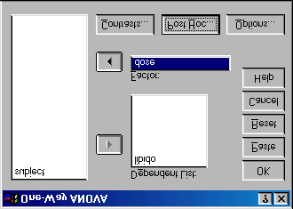
Running One-Way ANOVA on SPSS First, let’s conduct an ANOVA on the Viagra data. As with the data from last week (rugby injuries) we need to enter the data into the spreadsheet using a coding variable specifying to which of the three groups the score belongs. So, the data must be entered in two columns (one called dose which specifies how much Viagra the subject was given and one called libido which indicates the subject’s libido over the following week). You can code the variable dose any way you wish but I recommend something simple such as 1 = placebo, 2 = low dose and 3 = high dose. To conduct one-way ANOVA we have to first access the main dialogue box using the Analyze⇒Compare Means⇒One-way ANOVA This dialogue box has a space
where you can list one or more dependent variables and a second space to specify a grouping variable, or factor. Factor is another term for independent variable.
C8057(Research Methods 2): Contrasts and Post Hoc Tests Figure 1: Dialogue box for one-way ANOVA
For the Viagra data we need select only libido from the variable list and transfer it to the box labelled Dependent List by clicking on
. Then select the grouping variable dose and transfer it to the box Planned Comparisons Using SPSS If you click on
you access the dialogue box that allows you to conduct planned comparisons.
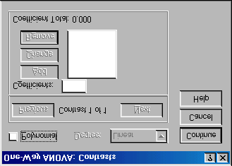
Figure 2: Dialogue box for conducting planned comparisons
section is for specifying trend analyses. If you want to test for trends in the data then tick the box labelled Polynomial. Once this box is ticked,
you can select the degree of polynomial you would like. The Viagra data has only three groups and so the highest degree of trend there can be is a quadratic
trend (see Field, 2000 Chapter 7). Now, it is important from the point of view of trend analysis that we have coded the grouping variable in a meaningful order. Now, we expect libido to be smallest in the placebo group, to increase in the low dose group and then to increase again in the high dose group. To detect a meaningful trend, we need to have coded these groups in ascending order. We have done this by coding the placebo group with the lowest value 1, the low dose group with the middle value 2, and the high dose group with the highest coding value of 3. If we coded the groups differently, this would influence both whether a trend is detected, and if by chance a trend is detected whether it is meaningful.
C8057(Research Methods 2): Contrasts and Post Hoc Tests
For the Viagra data there are only three groups and so we should select the polynomial option (
), and then select a quadratic degree by clicking on and then selecting quadratic. If a
quadratic trend is selected SPSS will test for both linear and quadratic trends. To conduct
planned comparisons we need to tell SPSS what weightings to assign to each group. The first step is to decide which comparisons you want to do and then what weights must be assigned to each group for
each of the contrasts (see Field, 2000 Chapter 7 p. 258–267). A sensible set of contrasts would be to compare the two experimental groups to the control group (Low dose + high dose vs. Placebo) as
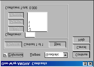
contrast 1, and then compare the low dose to the high dose in a second contrast. The weights for contrast 1 would be: –2 (placebo group), +1 (Low dose group), and +1 (high dose group). We will specify this contrast first. It is important to make sure that you enter the correct weighting for each
group, so you should remember that the first weight that you enter should be the weight for the first
group (that is, the group coded with the lowest value in the spreadsheet). For the Viagra data, the group coded with the lowest value was the placebo group (which had a code of 1) and so we should enter the weighting for this group first. Click in the box labelled Coefficients with the mouse and then
type ‘–2’ in this box and click on
. Next, we need to input the weight for the second group,
which for the Viagra data is the low dose group (because this group was coded in the spreadsheet with
the second highest value). Click in the box labelled Coefficients with the mouse and then type ‘1’ in this box and click on
. Finally, we need to input the weight for the last group, which for the Viagra
data is the high dose group (because this group was coded with the highest value in the spreadsheet). Click in the box labelled Coefficients with the mouse and then type ‘1’ in this box and click on
Figure 3: Contrasts dialogue box completed for the first contrast of the Viagra data.
Once you have inputted the weightings you can change or remove any one of them by using the mouse to select the weight that you want to change. The weight will then appear in the box labelled Coefficients where you can type in a new weight and then click on
any of the weights and remove it completely by clicking
. Underneath the weights SPSS calculates
the coefficient total, should equal zero (If you’ve used the correct weights). If the coefficient number is anything other than zero you should go back and check that the contrasts you have planned make
sense and that you have followed the appropriate rules for assigning weights. Once you have specified the first contrast, click on
. The weightings that you have just entered
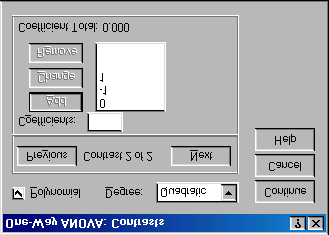
will disappear and the dialogue box will now read contrast 2 of 2. The weights for contrast 2 should be: 0 (placebo group), +1 (Low dose group), and -1 (high dose group). We can specify this contrast as before. Remembering that the first weight we enter will be for the placebo group, we must enter the value zero as the first weight. Click in the box labelled Coefficients with the mouse and then type ‘0’
C8057(Research Methods 2): Contrasts and Post Hoc Tests
. Next, we need to input the weight for the low dose by clicking in the box labelled
Coefficients and then typing ‘1’ and clicking on
. Finally, we need to input the weight for the high
dose group by clicking in the box labelled Coefficients and then typing ‘-1’ and clicking on
Figure 4: Contrasts dialogue box completed for the second contrast of the Viagra data
You should notice that the weights add up to zero as they did for contrast 1. It is imperative that you
remember to input zero weights for any groups that are not in the contrast. When all of the planned contrasts have been specified click on
Post Hoc Tests in SPSS Once we have told SPSS which planned comparisons we have done, we can choose to do some post hoc tests. In theory if we have done planned comparisons we should not need to do post hoc tests (because we have already tested the hypotheses of interest). Likewise, if we choose to conduct post
hoc tests then we should not need to do planned contrasts (because we have no hypotheses to test). However, for the sake of space we will conduct some post hoc tests on the Viagra data. Click on
in the main dialogue box to access the post hoc tests dialogue bo
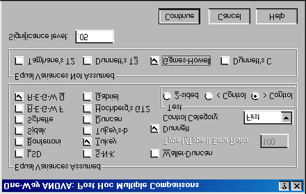
Figure 5: Dialogue box for specifying post hoc tests.
I recommend various post hoc procedures for various situations. The choice of comparison procedure will depend on the exact situation you have and whether it is more important for you to keep strict control over the familywise error rate or to have greater statistical power. However, some general guidelines can be drawn (see Field, 2000, p. 274–276). When you have equal sample sizes and
C8057(Research Methods 2): Contrasts and Post Hoc Tests
you are confident that your population variances are similar then use R-E-G-W-Q or Tukey because both have good power and tight control over the Type I error rate. If sample sizes are slightly different
then use Gabriel’s procedure because it has greater power, but if sample sizes are very different use Hochberg’s GT2. If there is any doubt that the population variances are equal then use the Games-
Howell procedure because this seems to generally offer the best performance. I recommend running the Games-Howell procedure in addition to any other tests you might select because of the
uncertainty of knowing whether the population variances are equivalent. For the Viagra data there are equal sample sizes and so we need not use Gabriel’s test. We should use Tukey’s test and R-E-G-W-Q and check the findings with the Games-Howell procedure. We have a specific hypothesis that both the high and low dose groups should differ from the placebo group and
so we could use Dunnett’s test to examine these hypotheses. Once you have
selected Dunnett’s test, you can change the control category (the default is to use the last category) to specify that the first category be used as the control category (because the placebo group was coded with the lowest value). You can also choose whether
), or a one-tailed test. If you choose a one-tailed test then you must
predict whether you believe that the mean of the control group will be less than the experimental
) or greater than the experimental groups (
These are all of the post hoc tests that need to be specified and when the completed dialogue box
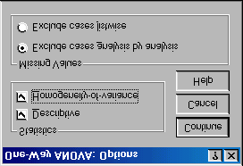
Options The options for one-way ANOVA are fairly straightforward. First you can ask for some descriptive statistics, which will display a table of the means, standard deviations, standard errors, ranges and confidence intervals for the means of each group. This is a useful option to select because it assists in
interpreting the final results. A vital option to select is the homogeneity of variance tests. As with the t-test, there is an assumption that the variances of the groups are equal and selecting this option tests
that this assumption has been met. SPSS uses the Levene test, which tests the hypothesis that the variances of each group are equal.
Figure 6: Options for One-Way ANOVA
data with a line superimposed to show the general trend of the means across groups. The line that joins the means seems to indicate a linear trend in that as the dose of Viagra increases so does the mean level of libido.
C8057(Research Methods 2): Contrasts and Post Hoc Tests Figure 7: Error bar chart of the Viagra data
One important part of the output is a summary table of Levene’s test. This test is designed to test the
null hypothesis that the variances of the groups are the same. It is an ANOVA conducted on the absolute differences between the observed data and the mean from which the data came. In this case,
Levene’s test is therefore testing whether the variances of the three groups are significantly different. If
Levene’s test is significant (i.e. the value of sig. is less than 0.05) then we can say that the variances are
significantly different. This would mean that we had violated one of the assumptions of ANOVA and we would have to take steps to rectify this matter. This most common way to rectify differences
between group variances is to transform all of the data. If the variances are unequal, they can sometimes be stabalised by taking the square root of every value of the dependent variable and then re-analysing these transformed values (see Howell, 1997, p. 323-329). However, for these data the
variances are very similar (hence the high probability value), in fact, if you look at some descriptive statistics you’ll see that the variances of the placebo and low dose groups are identical.
Test of Homogeneity of Variances SPSS Output 1
group effects (effects due to the experiment) and within group effects (this is the unsystematic variation in the data). The between group effect is further broken down into a linear and quadratic component and these components are the trend analyses described earlier. The between-group effect labelled combined is the overall experimental effect. In this row we are told the sums of squares for the model (SSM = 20.13). The sum of squares and mean squares represent the experimental effect. This overall effect is then broken down because we asked SPSS to conduct trend analyses of these data (we will
return to these trends in due course). Had we not specified this in sectio rows of the summary table would not be produced. The row labelled within group gives details of the unsystematic variation within the data (the variation due to natural individual differences in libido). The table tells us how much unsystematic variation exists (the residual sum of squares, SSR). It then gives the average amount of unsystematic variation, the mean squares (MSR). The test of whether the group
1 The interested reader might like to try this out. Simply create a new variable called diff (short for difference) which is each score subtracted from the mean of the group in which that score belongs. Then remove all of the minus signs (so, take the absolute value of diff) and conduct a one-way ANOVA with dose as the independent variable and diff as the
dependent variable. You’l find that the F-ratio for this analysis is 0.092, which is significant at p = 0.913!
C8057(Research Methods 2): Contrasts and Post Hoc Tests
means are the same is represented by the F-ratio for the combined between-group effect. The value of this ratio is 5.12. Finally SPSS tells us whether this value is likely to have happened by chance. The final
column labelled sig. Indicates how likely it is that an F-ratio of that size would have occurred by chance. In this case, there is a probability of 0.025 that an F-ratio of this size would have occurred by
chance (that’s only a 2.5% chance!). Social scientists use a cut of point of 0.05 as their criterion for statistical significance. Hence, because the observed significance value is less than 0.05 we can say that
there was a significant effect of Viagra. However, at this stage we still do not know exactly what the
effect of Viagra was (we don’t know which groups differed).
SPSS Output 2
Knowing that the overall effect of Viagra was significant, we can now look at the trend analysis. The
trend analysis breaks down the experimental effect into that which can be explained by a linear relationship and that which can be explained through a quadratic relationship. First let’s look at the linear component. This comparison tests whether the means increase across groups in a linear way. Again the sum of squares and mean squares are given, but the most important things to note are the value of the F-ratio and the corresponding significance value. For the linear trend the F-ratio is 9.97 and
this value is significant at a 0.008 level of significance. Therefore we can say that as the dose of Viagra increased from nothing to a low dose to a high dose, libido increased proportionately. Moving onto the quadratic trend, this comparison is testing whether the pattern of means is curvilinear (i.e. is
represented by a curve with one bend in). The error bar graph of the data strongly suggests that the means cannot be represented by a curve and the results for the quadratic trend bear this out. The F-ratio for the quadratic trend is nonsignificant (in fact, the value of F is less than 1, which immediately indicates that this contrast will not be significant
Output for Planned Comparisons In sectiold SPSS to conduct two planned comparisons: one to test whether the control
group was different to the two groups who received Viagra, and one to see whether the two doses of planned comparisons that we requested for the Viagra data. The first table displays the contrast coefficients; these values are the
contrasts are comparing what they are supposed to! As a quick rule of thumb, remember that when we do planned comparisons we arrange the weights such that we compare any group with a positive weight against any group with a negative weight. Therefore, the table of weights shows that contrast 1
compares the placebo group against the two experimental groups, and contrast 2 compares the low dose group with the high dose group. It is useful to check this table to make sure that the weights that we entered into SPSS correspond to the weights we intended to enter into SPSS!
C8057(Research Methods 2): Contrasts and Post Hoc Tests Contrast Coefficients Contrast Tests SPSS Output 3
The second table gives the statistics for each contrast. The first thing to notice is that statistics are
produced for situations in which the group variances are equal, and when they are unequal. If Levene’s test was significant then you should read the part of the table labelled equal variances not assumed. However, for these data Levene’s test was not significant and we can therefore use the part of the table labelled equal variances assumed. The table tells us the value of the contrast itself, which is the weighted sum of the group means. This value is obtained by taking each group mean, multiplying it by the weight for the contrast of interest, and then adding these values together. The table also gives the
standard error of each contrast and a t-statistic. The t-statistic is derived by dividing the contrast value by the standard error (
1 47 and is compared against critical values of the t-distribution. The
significance value of the contrast is given the final column and this value is two-tailed. Using the first contrast as an example, if we had used this contrast to test the general hypothesis that the experimental groups would differ from the placebo group, then we should use this two-tailed value. However, in reality we tested the hypothesis that the experimental groups would increase libido above the levels seen in the placebo group: this hypothesis is one-tailed. Provided the means for the
groups bare out the hypothesis we can divide the significance values by two to obtain the one-tailed probability. Hence, for contrast 1, we can say that Viagra significantly increased libido compared to the control groups (p = 0.0145). For contrast 2 we also had a one-tailed hypothesis (that a high dose of
Viagra would increase libido significantly more than a low dose) and the means bare this out. The significance of contrast two tells us that a high dose of Viagra increased libido significantly more than a low dose ( p(one −tailed) 0065
0 0345 ). Notice that had we not had a specific hypothesis regarding the
which group would have the highest mean then we would have had to conclude that the dose of Viagra had no significant effect on libido. For this reason it can be important as scientists that we
generate hypotheses before collecting any data because this is a more powerful method of scientific discovery. In summary, we have so far seen that there is an overall effect of Viagra on libido. Furthermore, the planned contrasts have revealed that having Viagra significantly increases libido compared to a control group (contrast1) and that having a high dose of Viagra significantly increases libido compared to a low
dose (contrast 2). 2 For the first contrast this value is (
C8057(Research Methods 2): Contrasts and Post Hoc Tests Output for Post Hoc Tests If we had no specific hypotheses about the effect that Viagra might have on libido then we could carry out post hoc tests to compare all groups of subjects with each other. In fact, we asked SPSS to do this
(see section and the results of this analysis are shown in SPSS Output 4. This table shows the results of Tukey’s test (known as Tukey’s HSD the Games-Howell procedure, and Dunnett’s test; which
were all specified earlier on. If we look at Tukey’s test first (because we have no reason to doubt that the population variances are unequal) it is clear from the table that each group of subjects is compared
with all of the remaining groups. For each pair of groups the difference between group means is displayed, the standard error of that difference, the significance level of that difference and a 95% confidence interval. First of all, the placebo group is compared to the 1 dose group and reveals a
nonsignificant difference (Sig. is greater than 0.05), but when compared to the high dose group there is
a significant difference (Sig. is less than 0.05). This finding is interesting because our planned comparison showed that any dose of Viagra produced a significant increase in libido, yet these comparisons indicate that a low dose does not. Why is there this contradiction (have a think about
this question before you read on — anyone wanting an answer can ask me)? The low dose group is compared to both the placebo group and the high dose group. The first thing to note is that the contrast involving the low dose and placebo group is identical to the one described previously. The only new information is the comparison of the two experimental conditions. The
group means differ by 2.8 which is not significant. This result also contradicts the planned comparisons (remember that contrast 2 compared these groups and found a significant difference). Think why this contradiction might exist (again, you can ask me for an answer if required).
Multiple Comparisons
The mean difference is significant at the .05 level.
a. Dunnett t-tests treat one group as a control, and compare all other groups against it. SPSS Output 4
3 The HSD stands for Honestly Significant Difference, which has a slightly dodgy ring to it if you ask me!
C8057(Research Methods 2): Contrasts and Post Hoc Tests
The rest of the table describes the Games-Howell tests and a quick inspection reveals the same pattern of results: the only groups that differed significantly were the high dose and placebo groups.
These results give us confidence in our conclusions because even if the populations variances are not equal (which seems unlikely given that the sample variances are very similar), then the profile of results
still holds true. Finally, Dunnett’s test is described and you’ll hopefully remember that we asked the computer to compare both experimental groups against the control using a 1-tailed hypothesis that
the mean of the control group would be smaller than both experimental groups. Even as a one-tailed
hypothesis levels of libido in the low dose group are equivalent to the placebo group. However, the high dose group has a significantly higher libido than the placebo group.
Another Example
Use the data from last week’s handout (rugby injuries) to conduct planned comparisons testing the hypotheses that: 1. Tonga cause more injuries than all of the other teams. 2. Japan cause less injuries than Wales and New Zealand 3. Wales and New Zealand are no different in terms of the injuries inflicted. Show the results to your seminar tutor.
This handout contains material from: Field, A. P. (2000). Discovering statistics using SPSS for Windows: advanced techniques for the beginner. London: Sage. So, it is Andy Field (2000) — please consult this book for more detail. To order a copy go to
Member Drug Formulary Alphabetical Listing 2008 The Member Drug Formulary is an alphabetical list of approved medicines covered by your benefit plan. In the Member Drug Formulary, generic drugs are listed by their generic name and begin with lower case letters. You will pay the lowest copay when you buy generic drugs. Formulary brand drugs are listed alphabetically by brand name. The nam
Safer Britain, Safer WorldThe decision not to replace Trident The decision on whether or not to replace Britain’s nuclear weapons system must be taken on the basis of what will most contribute to the security of the British people. A decision not to replace Trident will best meet that requirement. It will strengthen the international disarmament and non-proliferation regime


 C8057(Research Methods 2): Contrasts and Post Hoc Tests
Figure 1: Dialogue box for one-way ANOVA
C8057(Research Methods 2): Contrasts and Post Hoc Tests
Figure 1: Dialogue box for one-way ANOVA 


 C8057(Research Methods 2): Contrasts and Post Hoc Tests
For the Viagra data there are only three groups and so we should select the polynomial option (
), and then select a quadratic degree by clicking on and then selecting quadratic. If a
quadratic trend is selected SPSS will test for both linear and quadratic trends. To conduct
planned comparisons we need to tell SPSS what weightings to assign to each group. The first step is to decide which comparisons you want to do and then what weights must be assigned to each group for
each of the contrasts (see Field, 2000 Chapter 7 p. 258–267). A sensible set of contrasts would be to compare the two experimental groups to the control group (Low dose + high dose vs. Placebo) as
contrast 1, and then compare the low dose to the high dose in a second contrast. The weights for contrast 1 would be: –2 (placebo group), +1 (Low dose group), and +1 (high dose group). We will specify this contrast first. It is important to make sure that you enter the correct weighting for each
group, so you should remember that the first weight that you enter should be the weight for the first
group (that is, the group coded with the lowest value in the spreadsheet). For the Viagra data, the group coded with the lowest value was the placebo group (which had a code of 1) and so we should enter the weighting for this group first. Click in the box labelled Coefficients with the mouse and then
type ‘–2’ in this box and click on
. Next, we need to input the weight for the second group,
which for the Viagra data is the low dose group (because this group was coded in the spreadsheet with
the second highest value). Click in the box labelled Coefficients with the mouse and then type ‘1’ in this box and click on
. Finally, we need to input the weight for the last group, which for the Viagra
data is the high dose group (because this group was coded with the highest value in the spreadsheet). Click in the box labelled Coefficients with the mouse and then type ‘1’ in this box and click on
Figure 3: Contrasts dialogue box completed for the first contrast of the Viagra data.
C8057(Research Methods 2): Contrasts and Post Hoc Tests
For the Viagra data there are only three groups and so we should select the polynomial option (
), and then select a quadratic degree by clicking on and then selecting quadratic. If a
quadratic trend is selected SPSS will test for both linear and quadratic trends. To conduct
planned comparisons we need to tell SPSS what weightings to assign to each group. The first step is to decide which comparisons you want to do and then what weights must be assigned to each group for
each of the contrasts (see Field, 2000 Chapter 7 p. 258–267). A sensible set of contrasts would be to compare the two experimental groups to the control group (Low dose + high dose vs. Placebo) as
contrast 1, and then compare the low dose to the high dose in a second contrast. The weights for contrast 1 would be: –2 (placebo group), +1 (Low dose group), and +1 (high dose group). We will specify this contrast first. It is important to make sure that you enter the correct weighting for each
group, so you should remember that the first weight that you enter should be the weight for the first
group (that is, the group coded with the lowest value in the spreadsheet). For the Viagra data, the group coded with the lowest value was the placebo group (which had a code of 1) and so we should enter the weighting for this group first. Click in the box labelled Coefficients with the mouse and then
type ‘–2’ in this box and click on
. Next, we need to input the weight for the second group,
which for the Viagra data is the low dose group (because this group was coded in the spreadsheet with
the second highest value). Click in the box labelled Coefficients with the mouse and then type ‘1’ in this box and click on
. Finally, we need to input the weight for the last group, which for the Viagra
data is the high dose group (because this group was coded with the highest value in the spreadsheet). Click in the box labelled Coefficients with the mouse and then type ‘1’ in this box and click on
Figure 3: Contrasts dialogue box completed for the first contrast of the Viagra data. 


 C8057(Research Methods 2): Contrasts and Post Hoc Tests
. Next, we need to input the weight for the low dose by clicking in the box labelled
Coefficients and then typing ‘1’ and clicking on
. Finally, we need to input the weight for the high
dose group by clicking in the box labelled Coefficients and then typing ‘-1’ and clicking on
Figure 4: Contrasts dialogue box completed for the second contrast of the Viagra data
C8057(Research Methods 2): Contrasts and Post Hoc Tests
. Next, we need to input the weight for the low dose by clicking in the box labelled
Coefficients and then typing ‘1’ and clicking on
. Finally, we need to input the weight for the high
dose group by clicking in the box labelled Coefficients and then typing ‘-1’ and clicking on
Figure 4: Contrasts dialogue box completed for the second contrast of the Viagra data 


 C8057(Research Methods 2): Contrasts and Post Hoc Tests
you are confident that your population variances are similar then use R-E-G-W-Q or Tukey because both have good power and tight control over the Type I error rate. If sample sizes are slightly different
then use Gabriel’s procedure because it has greater power, but if sample sizes are very different use Hochberg’s GT2. If there is any doubt that the population variances are equal then use the Games-
Howell procedure because this seems to generally offer the best performance. I recommend running the Games-Howell procedure in addition to any other tests you might select because of the
uncertainty of knowing whether the population variances are equivalent. For the Viagra data there are equal sample sizes and so we need not use Gabriel’s test. We should use Tukey’s test and R-E-G-W-Q and check the findings with the Games-Howell procedure. We have a specific hypothesis that both the high and low dose groups should differ from the placebo group and
so we could use Dunnett’s test to examine these hypotheses. Once you have
selected Dunnett’s test, you can change the control category (the default is to use the last category) to specify that the first category be used as the control category (because the placebo group was coded with the lowest value). You can also choose whether
), or a one-tailed test. If you choose a one-tailed test then you must
predict whether you believe that the mean of the control group will be less than the experimental
) or greater than the experimental groups (
These are all of the post hoc tests that need to be specified and when the completed dialogue box
Options
C8057(Research Methods 2): Contrasts and Post Hoc Tests
you are confident that your population variances are similar then use R-E-G-W-Q or Tukey because both have good power and tight control over the Type I error rate. If sample sizes are slightly different
then use Gabriel’s procedure because it has greater power, but if sample sizes are very different use Hochberg’s GT2. If there is any doubt that the population variances are equal then use the Games-
Howell procedure because this seems to generally offer the best performance. I recommend running the Games-Howell procedure in addition to any other tests you might select because of the
uncertainty of knowing whether the population variances are equivalent. For the Viagra data there are equal sample sizes and so we need not use Gabriel’s test. We should use Tukey’s test and R-E-G-W-Q and check the findings with the Games-Howell procedure. We have a specific hypothesis that both the high and low dose groups should differ from the placebo group and
so we could use Dunnett’s test to examine these hypotheses. Once you have
selected Dunnett’s test, you can change the control category (the default is to use the last category) to specify that the first category be used as the control category (because the placebo group was coded with the lowest value). You can also choose whether
), or a one-tailed test. If you choose a one-tailed test then you must
predict whether you believe that the mean of the control group will be less than the experimental
) or greater than the experimental groups (
These are all of the post hoc tests that need to be specified and when the completed dialogue box
Options 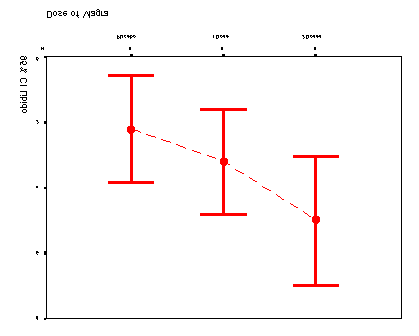 C8057(Research Methods 2): Contrasts and Post Hoc Tests
Figure 7: Error bar chart of the Viagra data
C8057(Research Methods 2): Contrasts and Post Hoc Tests
Figure 7: Error bar chart of the Viagra data