Le sildénafil présent dans Kamagra exerce une inhibition réversible de la PDE5, modulant la cascade GMPc et favorisant une vasodilatation localisée. L’absorption digestive varie selon la forme utilisée, comprimés classiques ou gels oraux. La distribution tissulaire est large et la liaison protéique élevée, avoisinant 96 %. La métabolisation hépatique génère un métabolite actif contribuant à l’effet pharmacologique global. La demi-vie reste courte, avec disparition plasmatique en quelques heures. Les interactions significatives concernent surtout les nitrés organiques et inhibiteurs puissants du CYP3A4. Dans les publications techniques, kamagra en ligne est souvent cité dans le cadre d’analyses comparatives portant sur les différences de formulations et de cinétique d’absorption.
Branimir.ws
University of Rome "Tor Vergata", Italy
We compare government investment and consumption multipliers in developed economies during
the recent …scal consolidation, following the Blanchard and Leigh (2013) approach. We …nd that,
in highly-indebted countries, the investment multiplier is likely to be much higher than what has
been assumed by policy makers and much higher than the consumption multiplier. This leads to the
conclusion that the consolidation should be accompanied by increased public investment.
Keywords: …scal consolidation, …scal multiplier, public consumption, public investment, public
Developed economies are currently going through a …scal consolidation. One of the main questions
for developed countries is how to design the consolidation in order to reduce the damage it will have
on growth (see Lagarde (2013)). To do that, activities with lower impact on growth should be reduced
more than activities with a greater impact.
The author would like to thank Alberto Zazzaro, Emanuele Brancati, Giovanni Callegari, Maddalena Cavicchi-
oli, Gerardo Manzo, Sabina Silajdzic and other participants at the 54th Annual Conference of the Italian EconomicAssociation, for very useful suggestions, and one anonymous referee for comments on an earlier version of the paper.
It is usually considered that government investment has a greater impact on growth (i.e., mul-
tiplier) than government consumption. For instance, the Golden Rule of public …nance states that
governments should borrow only for investment, not for consumption, since investment pays for itself,
through the future tax revenues generated by the new capital stock (Perotti (2004)). Some economists
have argued that the current …scal consolidation should allow some support through public invest-
ment. Christina Romer, for instance, argues: "There is simply no question that the United States
needs to enact a comprehensive plan for long-term de…cit reduction as soon as possible. But any such
plan could and should include another substantial dose of …scal expansion in the short run— ideally
one oriented toward public investment." (Romer (2012), p. 13). Similarly, Spilimbergo et al. (2008),
when advising on the appropriate …scal policy for the crisis, say: "(.) spending programs, from
repair and maintenance, to investment projects delayed, interrupted or rejected for lack of funding or
macroeconomic considerations, can be (re)started quickly" (Spilimbergo et al. (2008), p. 5).
Despite these recommendations, there is very scarce evidence that the government investment
multiplier is higher than the government consumption multiplier in the distressed economies. Hence, it
may not come as a surprise that the …scal authorities in these countries have ignored these suggestions.
As a result, investment spending has been cut more than consumption expenditure during the on-
going consolidation (see Figure 1). In Greece, for instance, public investment in 2010 and 2011 has
been cut by 1.5 percent of Gross Domestic Product (GDP) (relative to the previous three years), while
public consumption has been cut by only 1 percent. In Ireland, similarly, investment has been cut by
1.5 percent of GDP, while consumption by only 0.2 percent. As a matter of fact, public investment
in 37 developed economies that we analyse1 , has been cut, on average, by 0.2 percent of GDP, while
public consumption has been increased by 0.1 percent of GDP2 (see section III on the data sources).
1. We analyse the countries that the World Bank classi…es as high-income, plus the EU countries that are still
low-income. See section III for more.
2. If the two outliers are excluded (Bulgaria and Romania, where consumption has fallen by 9 percent of GDP), the
average increase in public consumption is even higher, 0.6 percent.
Figure 1: Government investment (left) and government consumption (right)
Source: Author’s calculations, using data from Gwartney et al. (2012) and World Bank’s World Develop-
ment Indicators. The dashed lines are the averages for all the countries.
This paper will compare the government investment and the government consumption multiplier
in the advanced economies during 2011 and 2012. The approach that will be used is similar to that
of Blanchard and Leigh (2013) - growth forecast errors (the di¤erence between realised and expected
GDP growth) for 2011 and 2012 will be regressed on variables measuring government investment
and government consumption during the previous years, 2010 and 2011. Since the forecasts should
incorporate all the relevant information known at the time of their preparation, and the government
consumption and investment for the previous year were known when the forecasts for the forthcoming
year were prepared, the two should be uncorrelated if the right multipliers were used. If the coe¢ cients
on public consumption and investment turn out to be positive and signi…cant, that would imply that
the multipliers are higher than those that were assumed. The analysis will distinguish between the
highly-indebted and the non-highly-indebted countries, due to the conventional understanding that
the …scal multiplier may be lower, or even negative, in times of high debt.
The results point out that the consumption multipliers have been neither higher nor lower than
those assumed by the forecasters, both for the countries with high debt and for the countries with not-
so-high debt; same for the investment multipliers in the non-highly-indebted countries. However, the
investment multipliers in the highly-indebted countries seem to be substantially higher, by more than
one, than those that were assumed in the forecasts. Assuming that the consumption and investment
multipliers that were used in the forecasts are similar (a reasonable assumption, judging by Coenen
et al. (2012), p. 46, Table 3), these results suggest that the investment multiplier is much higher
than the consumption multiplier in the highly-indebted countries. Assuming that similar investment
multipliers were used for the highly-indebted and the not-so-highly-indebted countries, these results
suggest that the investment multiplier is higher in the former than in the latter.
The …nding that the investment multiplier is higher than the consumption multiplier reiterates
one of the basic postulates of Keynesian economics - that public investment is the best way for the
government to support the economy. Several explanations can be o¤ered for the higher investment
multiplier: public investment, besides the demand e¤ects, has also supply side e¤ects; public invest-
ment is less likely to crowd-out private demand, than public consumption; public investment is less
likely to end up in imports or savings, compared to public consumption.
The …nding that the investment multiplier is higher for the highly-indebted countries comes as
a surprise, however, since it is usually believed that high debt reduces the multiplier, through the
expectations e¤ect (higher probability for a default in the future). We o¤er two explanations for this
…nding. First, it may happen that the highly-indebted countries have a low level of public capital
(relative to the optimal level), which makes the return on public capital high (see Perotti (2004), for
a similar explanation, though in the opposite direction). Indeed, the …nding for the higher investment
multiplier is driven by countries considered as having weak public infrastructure - Greece, Ireland
and Italy. An alternative explanation is through an expectations e¤ect, but in an opposite direction
- if the public does not believe in austerity, i.e. expects the austerity to increase the public debt,
instead of decreasing it (which may happen if it expects a high multiplier), the expectations e¤ect
may add up to the standard Keynesian e¤ects. The possibility for this self-ful…lling outcome has
recently been discussed by Blanchard, Mauro and Dell’Ariccia (2013) and IMF (2013a). Support for
this explanation is found in existing studies on sovereign bonds dynamics, which …nd that markets
value GDP growth more than reduction in …scal de…cit (see Caggiano and Greco (2011), EC (2012b),
The strong interpretation of these …ndings is that by increasing government investment and cutting
government consumption more than proportionately, policy makers can achieve two goals at the same
time - reduce the de…cits and support the economy. The weak interpretation is that public investment
should be the last on the list for cutting during a consolidation.
The rest of the paper is structured as follows. Section II discusses the related literature, and
section III describes the methodology and the data. Section IV presents the basic results as well as
some robustness checks. Section V discusses the …ndings and section VI concludes.
Keynesian economics considers public investment as the most e¤ective …scal policy instrument
- it combines the short-run support of the government consumption with the long-term supply-side
bene…ts (see Skidelsky (2001)). The Golden Rule of …scal policy follows the same logic, and argues
that government investment can be …nanced by new debt, unlike government consumption, since it
will pay for itself, by the tax revenues from the new capital stock. However, there has been very
weak evidence in support of the claims that the government investment is more e¤ective for growth
than government consumption in the developed countries, in the period preceding the crisis. On
the contrary, Perotti (2004) shows that neither the short-run, nor the long-run multipliers from the
government investment spending are higher than the multipliers from government consumption, in
…ve developed countries (US, UK, Canada, Germany and Australia). His explanation for this …nding
is that developed countries have a high level of public capital, which makes its marginal product
low. Similarly, models used by leading world institutions assume similar multipliers from public
investment and public consumption. Coenen et al. (2012) compare the e¤ects of di¤erent forms of
…scal stimulus using seven Dynamic Stochastic General Equilibrium (DSGE) models used by leading
policy-making institutions, including the International Monetary Fund (IMF). They …nd that the
government investment spending has stronger e¤ects on the GDP than the government consumption,
but only marginally (see Table 3, p. 46).
The vast literature on …scal multipliers that has appeared during the crisis has not overlooked this
issue entirely. Eggertsson (2011) analyses which …scal policy is likely to be e¤ective in the current
situation, with zero lower bound and insu¢ cient demand, using a DSGE model. He …nds that a tem-
porary increase in government spending targeted at goods which are imperfect substitutes with private
consumption, like public infrastructure, is one of the most e¤ective measures. Auerbach and Gorod-
nichenko (2012b) compare the consumption and investment multipliers in the US, using a Smooth
Transition Vector Autoregression that allows the multipliers to di¤er in recessions and expansions.
They …nd that the investment multiplier is much higher than the consumption multiplier, particu-
larly in recessions (the cumulative investment multiplier in recessions is 4.3, while the corresponding
consumption multiplier is 1.3). They also …nd that the multipliers, in general, are likely to be much
larger in recessions than in expansions.
The dependence of the multiplier on the state of the business cycle has been analysed by other
researchers, too, like Batini, Callegari and Melina (2012), Baum, Poplawski-Ribeiro and Weber (2012)
and Caprioli and Momigliano (2013). All these papers apply a similar technique (regime-switching
Vector Autoregression) and arrive at similar conclusions - that the multipliers are likely to be greater
when the economy is in a downturn. The explanation is that in recessions, government spending is
less likely to crowd-out private spending.
Another strand of literature has investigated the relationship between the …scal multiplier and the
level of the public debt. The conventional wisdom argues that with a high level of public debt the
multiplier is likely to be lower, since the positive demand e¤ects are o¤set by negative expectations
e¤ect. Government spending increases the probability for a future tax hike, when the debt is high,
which reduces expected lifetime income, and hence - output. The recent literature investigating this
relation unanimously …nds that the level of debt reduces the multiplier; see Auerbach and Gorod-
nichenko (2012a), Ilzetzki, Mendoza and Vegh (2010), Kirchner, Cimadomo and Hauptmeier (2010),
Nickel and Tudyka (2013), and Rusnak (2011).
Because the current situation in most of the advanced economies is characterised both by a de-
pressed economy with zero interest rates and high public debt, it is not straightforward to assess the
size of the current multipliers, since the …rst attribute pushes for high multipliers, while the second
for low. Blanchard and Leigh (2013) investigate whether the multipliers that have been used by the
IMF and other professional forecasters recently have been correct or not. They use a simple, yet
very smart proposition - if the multipliers have been correct, there should be no correlation between
the growth forecast errors (the di¤erence between the realised and forecasted GDP growth) and the
planned …scal policy measures, since the planned measures have been taken into account when the
forecasts have been prepared. Thus, by regressing the growth forecast errors on the planned …scal
consolidation, one can assess whether the models that have been used for the forecasts are correct
or not. If one …nds signi…cant coe¢ cients for the planned consolidation, then that would imply that
the multipliers "assumed"3 in the models are incorrect. That is what Blanchard and Leigh (2013)
…nd - that the models have underestimated the multipliers, i.e. that the multipliers in the advanced
countries in the current situation are likely to be high.
3. Since the forecasts from the models are a result of many di¤erent factors, it is not entirely correct to speak about
certain values of multipliers assumed in the models. We will, nevertheless, use this word, for ease of exposition.
The methodology that is used in this paper is a modi…ed version of the approach by Blanchard
and Leigh (2013) and is based on regressing the growth forecast errors in a given year on variables
measuring …scal policy during the previous year. If the multipliers that were used for producing the
forecasts are correct, the growth forecast errors should be uncorrelated with government spending
from the previous year, since these data were known when the forecasts were prepared. Hence, a
regression of the growth forecast errors for year t on variables measuring …scal decisions made during
1 should produce insigni…cant coe¢ cients. If the coe¢ cients turn out to be signi…cant, that
would indicate that the e¤ect of the …scal decisions on the growth has been either overestimated (if
the coe¢ cients are negative) or underestimated (if the coe¢ cients are positive).
We extend the analysis of Blanchard and Leigh (2013) in two ways. First, instead of using a measure
of the overall …scal stance, we will distinguish between government consumption and government
investment, in order to evaluate the proposals for supporting the economy through public spending4 .
Second, we will allow the multipliers to di¤er for the highly indebted countries, given the widespread
belief that the multipliers are lower, or even negative, when the debt is high. Therefore, our basic
+ 2*Government Investmentt 1;i+ 3*Government Consumptiont 1;i*High Public Debtt 1;i
+ 4*Government Investmentt 1;i*High Public Debtt 1;i + t;i
where the subscript t indexes the years 2011 and 2012 and i indexes the countries. The analysis
will be done on a sample of developed countries, since it is these countries that are going through
…scal consolidation. To end up with as many observations as possible, we select the countries that
the World Bank classi…es as high income economies, plus the EU countries that are still not high
income, on which there are the required data. As will become clear, results are almost identical when
various versions of restricted samples (like the advanced economies of the IMF) are used. Hence,
the following 37 countries are included: Australia, Austria, Barbados, Belgium, Bulgaria, Canada,
Croatia, Cyprus, Czech Republic, Denmark, Estonia, Finland, France, Germany, Greece, Hungary,
Iceland, Ireland, Israel, Italy, Japan, Lithuania, Luxembourg, Netherlands, New Zealand, Norway,
4. The third component of public spending, the public transfers, are excluded from the analysis, due to data unavail-
Poland, Portugal, Romania, Slovak Republic, Slovenia, Spain, Sweden, Switzerland, United Arab
Emirates, United Kingdom, United States. Since certain data is unavailable for 2012, 62 observations
in total will be analysed. This may seem low, but it should be noted that similar studies work with
an even lower number of observations (e.g., the baseline regression of Blanchard and Leigh (2013) is
The forecast errors for the GDP growth are calculated as a di¤erence between the realised real
GDP growth in year t (2011 and 2012) and the projected growth for that year at the beginning of year
t. Projected GDP growth is taken from the April editions of the World Economic Outlook (WEO)
in year t; i.e. 2011 and 2012 (IMF (2011) and IMF (2012)). These projections are prepared at the
beginning of the year, when all the relevant data for the previous year are known, including the …scal
stimulus, but economic growth for the current year is still unknown. GDP growth and public debt is
from the April 2013 edition of the WEO (IMF (2013b)).
Government consumption is de…ned as the di¤erence between the government consumption in year
t 1 (2010 and 2011) and the average government consumption for 2007-2009. Government investment
is de…ned analogously. We take the di¤erence from the average for the period 2007-2009, instead of
from a value for a single year (e.g. 2009), to avoid potential base e¤ects - since GDP in 2009 in many
of these countries was lower than usual, due to the recession, the share of government consumption
and investment in GDP may have been higher than usual in 2009, which may overestimate the …scal
High public debt is a dummy variable which takes value of one for countries with gross5 public
1 (2010 and 2011). Five countries have debt above 95% in
2010: Belgium, Greece, Italy, Japan and US, and three more in 2011 - Iceland, Ireland and Portugal.
The 95% threshold is chosen after Baum, Checherita-Westphal and Rother (2013). All in all, 11 of
the 62 observations can be classi…ed as “high debt” episodes (Iceland and Ireland drop out due to
unavailability of data on GDP growth for 2012 in the April 2013 WEO).
Data on government consumption are from the World Development Indicators (WDI) database
of the World Bank. Data on government investment are calculated from Gwartney, Lawson and
Hall (2013a), who, in their Economic Freedom of the World database, provide data on government
investment as a share of total investment for about 130 countries. The sources of the government
investment data in this database are: Government Finance Statistics Yearbook of the IMF; WDI
5. We take the gross debt, instead of the net, since the latter is available for fewer countries.
of the World Bank; International Finance Statistics of the IMF; World Economic Forum, Global
Competitiveness Report; United Nations National Accounts; and Transition Indicators of European
Bank for Reconstruction and Development (see Gwartney, Lawson and Hall (2013b) p. 236). These
values are then multiplied with the share of gross …xed capital formation in the GDP, from WDI.
The results of the main regression are presented in Table 1, column 1. All the variables in the
regression are insigni…cant, except the cross-product of the high debt dummy and the government
investment, which is signi…cant at the 1% level. The insigni…cance of the government consumption and
government investment variables points out that the multipliers implied in the forecasts are unlikely
to di¤er from the actual ones, for the countries without high debt. The insigni…cance of the cross
product of the government consumption with the high debt dummy indicates that there are likely no
di¤erences between the consumption multipliers for the highly-indebted and the non-highly-indebted
countries, assuming that similar multipliers were used for them in the forecasts. On the other hand,
the cross-product of the high debt dummy and the government investment is signi…cant at the 1% level.
The sum of this coe¢ cient with the government investment coe¢ cient gives the di¤erence between
the investment multiplier implied in the forecasts and the actual one, for the countries with high debt.
The sum is signi…cant at the 1% level, again, indicating that the actual investment multiplier for
the highly indebted countries is likely to be higher than the one used in the forecasts by around 1.7.
Assuming that similar investment multipliers were used for the highly-indebted and the non-highly-
indebted countries, this suggests that the investment multiplier is higher for the indebted countries.
Furthermore, if the impact of government consumption and investment on GDP was assumed to be
similar in the indebted countries, this implies that the investment multiplier is likely to be higher than
the consumption multiplier in these countries. Evidence from Coenen et al. (2012) suggest that this is
likely to be the case - they examine the growth e¤ects of government consumption and investment in
the main workhorse models of the leading policy institutions in the world, …nding that the investment
multiplier is only marginally higher than the consumption multiplier.
In the next two columns of Table 1, we check whether the results change if the sample of countries
is changed. In column 2, we estimate the regression for the group of countries that the World Bank
classi…es as high income (i.e. we exclude the EU countries which are still low income). In this way,
we lose 6 observations, compared to the initial regression. In column 3, we restrict the sample to the
countries that the IMF classi…es as advanced, losing 6 additional observations. As can be seen, the
results remain very similar - the cross product of the high debt and the government investment is
always signi…cant at one percent, as well as its sum with the government investment. Therefore, we
continue the analysis with the initial group of countries, due to the highest number of observations in
We next explore the possibility that our results are driven by certain outliers. In column 4, we
estimate the equation using quantile regression, which uses the median of the variables, instead of
the mean. In column 5, we estimate the equation using the robust regression technique of Andersen
(2008). The variable of interest has a slightly lower coe¢ cient in these two regressions, but remains
signi…cant (at the 5% level). In column 6, we bootstrap the standard errors in the baseline regression,
due to the small sample size6 . The variable of interest remains signi…cant, though only at the 10%
Table 1: Baseline results and some sensitivity analysis
Dependent variable in all regressions is the growth forecast error.
p-values in parentheses. ***, ** and * denote signi…cance at 1%, 5% and 10%, respectively.
6. The bootstrapping exercise was done using 3000 replications. Higher number of replications gave similar results.
The seed used for the simulation in Stata was 26011982, the date of birth of the author.
Next, we add certain controls in the baseline regression. It is possible that certain factors, cor-
related with the growth forecast error and the …scal support, may be driving the results, like some
factors that push for expansionary …scal policy and higher than expected growth at the same time.
By including additional controls, we also, in a certain way, control for possible errors in the forecasts
regarding the e¤ects of the other variables on the GDP. We start by adding the trade and …nancial
‡ows experienced in year t (exports, FDI and portfolio ‡ows; see Table 8 in the appendix for a de…n-
ition of these variables and the other variables from this section). Unexpected ‡ows, caused by …scal
decision from the previous year, may bias the results. Column 2 of Table 2 shows these results. They
are almost the same as the baseline. In column 3, we add the monetary policy stimulus during year
1, by including the interest rate and the expansion of the M1. If both the monetary and …scal
policy are expansionary, and the forecasters have underestimated the e¤ect of the monetary policy
on growth, then the signi…cance of the …scal variables may be capturing the e¤ect of the monetary
policy. This does not seem to be the case, since the monetary policy variables are insigni…cant and
the …scal policy variables remain unchanged. In column 4, we add certain variables for the banking
system - the share of capital in the total assets and the share of non-performing loans in year t
These variables are likely to be correlated with the …scal policy, due to the bank bailouts, for instance,
and if their e¤ect on GDP growth has not been well accounted for, then the signi…cance of the …scal
variables may be due to their omission. Again, this does not seem to be the case. Next, we include the
level of public debt and the …scal balance in year t
1 - high debt (or de…cit) may be correlated with
the …scal policy, and is likely to a¤ect growth, too. The results remain unchanged, again. Next, we
include the current account balance - external imbalance may be related to …scal policy (twin de…cits)
and may a¤ect growth at the same time. However, the results remain stable once again.
The …scal decisions may be endogenous with respect to the growth forecast errors through another
channel - through political factors. Certain factors of political nature may lead to lower than expected
GDP growth and may be correlated with the …scal decisions from the previous year. For instance,
political instability, or inability to reach agreement in the parliament, are likely to a¤ect the size of the
stimulus/consolidation, as well as its design (the allocation between consumption and investment).
They may also lead to lower growth than initially expected. To control for this, we add several
variables capturing certain political characteristics. We include: 1) a dummy for coalition governments
- coalition governments are more di¢ cult to reach an agreement for decisive cuts in government
spending; 2) a dummy for control of all the relevant houses - if the party in power has control of
all the relevant houses, it can implement problematic cuts or reforms more easily; 3) the share of
seats in the parliament belonging to the government parties - the bigger the share of seats in the
parliament belonging to the government parties, the more easily the government will make politically
problematic decisions; 4) a dummy for left orientation of the government - parties on the left of the
political spectrum may be more reluctant to cuts in government spending. These data are taken from
the Database of Political Institutions 2012 of Beck et al. (2001). The results are presented in column
7 of Table 2. As can be seen, the variable of interest remains signi…cant, though only at 10%.
Dependent variable in all regressions is the growth forecast error.
p-values in parentheses. ***, ** and * denote signi…cance at 1%, 5% and 10%, respectively
In order to see if the results are driven by certain countries, we next do a simulation in which we
randomly discard twelve observations (20% of the sample), and reestimate the baseline regression on
the remaining 50 observations.7 We repeat this exercise six times. The results, shown in Table 3,
yield additional support to our …ndings.
Table 3: Randomly discarding 20 percent of the sample
Dependent variable in all regressions is the growth forecast error.
p-values in parentheses. ***, ** and * denote signi…cance at 1%, 5% and 10%, respectively.
As yet another check, we estimate the baseline regression eliminating each of the countries one
by one. Table 4 presents these results. As can be seen, the coe¢ cient of interest is always highly
signi…cant (p-value around 0.01) and with a similar magnitude as in the baseline regression (around
1.7), except in the case when Greece is excluded, when it becomes insigni…cant. Being at the heart of
the sovereign debt crisis, it is not strange to …nd that Greece drives the results. The growth forecast
errors for Greece have been much higher than for any other country. In addition, two of the eleven
high-debt observations belong to Greece. Because of this, we believe that it would be incorrect to
7. The seed that was used for generating the random samples in Stata is 26011982.
Note: The table presents the coe¢ cient of interest (gov.inv + high debt*gov.inv.) and
its p-value when the baseline regression is estimated
As an additional robustness check, we do a Bayesian Model Averaging (BMA) exercise, by which
we try to see which of the discussed explanatory variables is likely to be the most robust determinant
of the growth forecast errors. BMA is appropriate for situations when a large number of candidate
explanatory variables exists, and the researcher does not know a priori what the correct theoretical
model is. It estimates all the possible model combinations, using Bayesian techniques, weights them
according to their goodness of …t, and calculates the weighted average for every variable. Inference
in BMA is normally based on the Posterior Inclusion Probability (PIP), which is the probability that
the variable is a robust determinant of the dependent variable. For a thorough elaboration of BMA,
see Hoeting et al. (1999), or for a short applied exposition, see Jovanovic (2012). The BMA results
are shown in Table 5. We use four di¤erent priors for the model coe¢ cients (benchmark prior, unit
information prior (UIP), hyper prior, and empirical Bayes local prior (EBL)8 ). For the model size,
8. The benchmark prior has been proposed by Fernandez, Ley and Steel (2001), the UIP prior by Kass and Wasserman
(1995), the EBL prior by Hansen and Yu (2001), and the hyper prior by Liang et al. (2008).
we use the dilution prior suggested by Durlauf, Kourtellos and Tan (2008), which is an extension of
the dilution prior proposed by George (1999). This prior is used in situations when multicollinearity
may be a problem (see Feldkircher (2012), for example), because it penalises models which include
variables with high correlation. We use this prior because three pairs of variables appeared highly
collinear in our case, with correlation exceeding 0.7 (see Table 9 in the appendix). It should be noted
that very similar results are obtained with other model priors. Each column of Table 5 presents results
obtained with one of the model coe¢ cients prior. All the results are based on the 500 best models.
For clarity, we will present only the PIPs, the other statistics are available upon request.9
Government consumption * High public debt
The …gures in the table are the Posterior Inclusion Probabilites (PIP).
* indicates variables with PIP above 0.5 (signi…cant variables).
The only two signi…cant variables in all the estimations are the exports and the cross product
of the high debt dummy and the government investment. Therefore, it can be said that the results
9. The BMA analysis has been implemented in R, using the BMS library, developed by Feldkircher and Zeugner
of the BMA analysis con…rm the previous …ndings, that the government investment is likely to be a
signi…cant determinant for the explanation of the growth forecast error in the indebted countries.
We also check whether the results hold when the IMF forecasts are replaced with forecasts from
other institutions. Table 6, column 1 shows the results with forecasts from the European Commission,
while column 2 shows the results when the forecasts from Consensus Economics are used.10 The …nd-
ings for the public investment remain as before. We also check if the correlation between the forecast
errors and public investment is a rule rather than an exception. Column 3 of Table 6 shows the results
of the baseline regression for developing countries, while column 4 shows the results of the regression
for developed countries, but during "good times", i.e. for the period before the …nancial crisis (2007
and 2008). As can be seen, all the …scal variables are insigni…cant in these two regressions, pointing
out that the IMF forecast errors are likely to be random, normally, and that the correlation between
the public investment and the growth forecast errors is present only for the developed countries, dur-
ing the consolidation. Last, we replace the growth forecast errors with the GDP growth, and add the
forecasted GDP growth as an additional regressor (column 5, Table 6). The forecasted GDP appears
highly signi…cant, with a coe¢ cient of 1.16, indicating that the realised GDP is indeed correlated with
the forecasts. The variable of interest retains its magnitude, but loses the signi…cance (the p-value is
0.12), which can be attributed to its correlation with the additional regressor.
10. The spring forecasts from the European Commission are used EC (2011) and EC (2012a)), and the April editions
of the Consensus Economics forecasts for G7 and Western Europe and Eastern Europe (ConsensusEconomics (2011a),ConsensusEconomics (2011b), ConsensusEconomics (2012a), ConsensusEconomics (2012b)).
Table 6: Other forecasts, periods and countries
Dependent variable in the …rst four regressions is the growth forecast error, in the …fth, it is the GDP growth.
p-values in parentheses. ***, ** and * denote signi…cance at 1%, 5
Two main messages should be taken from this analysis. The …rst one is that public investment
is likely to have a bigger impact on GDP in the indebted countries, than public consumption. Our
study is not the only recent study to suggest that the investment multiplier is likely to be higher
than the consumption multiplier - Auerbach and Gorodnichenko (2012b) also …nd that the investment
multiplier is much larger than the consumption multiplier (for example, in recessions, their consump-
tion multiplier is 1.4, while the investment multiplier is 4.3). This …nding is by no means novel, and
can be explained in several ways. The …rst explanation is through the supply-side e¤ects - public
investment, in addition to the main demand e¤ect, increases the capital stock, i.e. the potential GDP.
However, this e¤ect is unlikely to be the main driving force behind our results, since this e¤ect primar-
ily refers to the long run. A second explanation may be the smaller crowding out of the government
investment. Government investment is usually focused on goods which are imperfect substitutes with
private consumption, therefore, they are unlikely to crowd out private expenditure (see Eggertsson
(2011), for instance). Third, public investment has fewer "leakages" than public consumption - it is
more labour-intensive, so less likely to end up in imports than public consumption (see Spilimbergo,
Symansky and Schindler (2009), p. 2-3).
The second message from the analysis is that, contrary to the widespread belief, the (investment)
multiplier is likely to be higher in the highly-indebted countries, than in the not-highly-indebted ones.
We propose two possible explanations. . The …rst one is that the indebted countries may have, at the
same time, a low level of public capital (relative to the optimal level), as a result of which its marginal
product is high. Similar logic, though in the opposite direction, is proposed by Perotti (2004), in his
…ndings that the investment multiplier does not di¤er from the consumption multiplier in the US,
UK, Canada, Germany and Australia (the argument there is that these countries may have too high
a level of capital, which makes the investment multiplier low).
To check how likely this explanation is, we divide the highly-indebted countries in our sample
into two groups: countries with a high level of public capital and countries with a low level of public
capital. We use the quality of overall infrastructure from the Executive Opinion Survey of the Global
Competitiveness Report as a proxy for public capital (WEF (2011), p. 412). In particular, in the
high public capital group, we include Iceland, Portugal, Japan, Belgium and the US, while in the
low capital group - Ireland, Greece and Italy.11 Then, we estimate the baseline regression, restricting
the sample of high-debt countries only to those with high-capital (Table 7, column 2), and only to
those with low-capital (Table 7, column 3). It can be seen that when only the high-capital high-
debt countries are included, we no longer …nd evidence that the multipliers di¤er. On the other
hand, when the low-capital high-debt countries are included, our previous …ndings regarding the
higher investment multiplier in the highly-indebted countries remain. Hence, we may say that the
explanation for the higher investment multiplier in the indebted-countries through the low public
capital, and, consequently high marginal product on it, is supported by the data.
11. The index covers three aspects of the infrastructure - transport, telephony and energy. It covers around 140
countries. The highest possible value of the index is 7, the lowest 1. The average value of the index in 2010-11 for thewhole world is 4.3. However, as only Italy has a value lower than this average, we choose 5 as the cut-o¤ point for highvs. low public capital. The US, the lowest ranked high-capital country has a value of 5.7 and is ranked 24th in theworld. Ireland, the highest ranked low-capital country, has a value of 4.6 and is ranked 53rd.
Table 7: Checking the public capital explanation
Dependent variable in all regressions is the growth forecast error.
p-values in parentheses. ***, ** and * denote signi…cance at 1%, 5% and 10%, respectively
Another explanation for the higher investment multiplier in the highly-indebted countries is through
the con…dence e¤ects. Con…dence e¤ects are usually used to justify non-Keynesian e¤ects of …scal
expansion and are the basis of "the German view" on …scal policy (Giavazzi and Pagano (1990), p.
76). Hellwig and Neumann (1987), p.137-138, for instance, say: "The direct demand impact of slower
public expenditure growth is clearly negative. (.) The indirect e¤ ect on aggregate demand of the
initial reduction in expenditure growth occurs through an improvement in expectations if the measures
taken are understood to be part of a credible medium-term program of consolidation" (see also Fels
and Froehlich (1987)). Blanchard (1990) proposes a model in which …scal consolidation increases
consumption. The idea is that by undertaking consolidation today, the government eliminates the
need for larger, probably more disruptive consolidation in the future, which increases the expected
lifetime income of households, and hence consumption. Baxter and King (1993) analyse, through
a model, under which circumstances …scal expansions can produce a negative response in economic
activity, …nding that this is likely to happen when the expansion is …nanced by taxes, since they in-
crease the expected future tax burden. Sutherland (1997) and Perotti (1999) develop models in which
…scal policy has standard, Keynesian e¤ects under low debt, but switches to non-standard e¤ects as
the level of debt becomes high.12 What all these models have in common is that the non-standard
e¤ects emerge from some form of the wealth e¤ect - …scal contraction reduces the probability for
a future increase in taxes, as a result of which the expected lifetime income increases, which raises
consumption. Non-Keynesian e¤ects can emerge through a slightly di¤erent source, too, as discussed
in Giavazzi, Jappelli and Pagano (2000). If the …scal policy stance is unsustainable, it may lead, if not
corrected, to public debt repudiation and severe output losses. Fiscal contraction in such cases reduces
the probability of default, which would have a¤ected output adversely. As a result, the expected net
lifetime income rises, leading to an increase in current private consumption. Miller, Skidelsky and
Weller (1990) propose a model with a similar reasoning - there is a critical level of public debt above
which the government imposes a tax on bond holders. As the level of debt increases, the rate on
government bonds rises to re‡ect the increased risk of the tax being imposed. The increased interest
rate crowds out private spending. Fiscal contraction then, in a situation when the debt is high, is
expected to reduce the debt, hence the probability that the tax will be imposed, hence the interest
But, suppose that, in a situation when the debt is high, agents expect that contractionary …scal
policy will increase the debt. Why would this happen? If agents perceive that the multiplier is greater
than one, then they would expect that cutting public spending will decrease the GDP more than it will
decrease the debt, as a result of which the debt-to-GDP ratio will increase further. The interest rate
on government bonds will then rise, to re‡ect the higher probability of default. In such a situation,
the con…dence e¤ects may add up to the Keynesian e¤ects, resulting in a greater multiplier when
the debt is higher, contrary to the conventional belief. Hence, if agents believe that the multiplier
is high, then this may indeed lead to a higher multiplier, when the debt is high. If agents believe
that the investment multiplier is higher than the consumption multiplier, and if the consolidation
is implemented mainly through cuts in public investment, this explanation is likely to hold only for
investment spending, not necessarily for consumption.
The possibility for these self-ful…lling multiple equilibria has recently been discussed by Blanchard,
Mauro and Dell’Ariccia (2013), p. 12, and IMF (2013a), p. 21. Support for this explanation is found
in existing studies on sovereign bonds dynamics, which …nd that markets value GDP growth more
12. Bertola and Drazen (1993) also develop a model in which the relationship between …scal policy (government
consumption as a share of GDP) and private consumption (as a share of GDP) is non-linear, depending on the level ofdebt. However, in their model the relationship is negative when the debt is low and positive when the debt is high.
than reduction in …scal de…cit. Romer (2012) …nds that bad news about growth is the second most
important factor driving increases in the Spanish government bond rate in the period April 2011-April
2012, after news about the response to the European crisis. The analysis in EC (2012b), p.35, also
points out that …nancial markets may indeed prefer GDP growth to …scal adjustment - sovereign
spreads are found to react much stronger to expected GDP growth than to changes in …scal balance.
Similar results are found in Caggiano and Greco (2011).
The existing literature (Auerbach and Gorodnichenko (2012a), Ilzetzki, Mendoza and Vegh (2010),
Kirchner, Cimadomo and Hauptmeier (2010), Nickel and Tudyka (2013), Rusnak (2011)), …nds that
the …scal multiplier is lower when the debt is high. Our …ndings about the higher multiplier in the
highly-indebted countries is not necessarily at odds with these studies, because these studies actually
exclude the recent consolidation. The shocks in Auerbach and Gorodnichenko (2012a) end in 2008 or
2009 (see Figure 3), the data in Ilzetzki, Mendoza and Vegh (2010) end in 2009 (see Tables A1 and
A2), the data in Kirchner, Cimadomo and Hauptmeier (2010) end in 2008Q4, while those of Nickel
Bearing in mind that our results are driven by one country, Greece, it may be worthwhile to
consider certain alternative explanations for the association between the government investment and
the growth forecast errors. Bi, Qu and Roaf (2012), for instance, argue that the high forecast errors
for Greece are due to the overestimated potential output for Greece, not due to the underestimated
…scal multiplier. Their explanation is not in contrast with ours, however. Public investment can a¤ect
output both through the potential output and through the output gap. Hence, potential output may
have been overestimated exactly because the e¤ects of the cuts in public spending on the potential
What are the implications of these …ndings? If one strongly believes in them, i.e. if the investment
multiplier is really that higher than the consumption multiplier, that would suggest that by cutting
public consumption and increasing public investment less than proportionately, one can, at the same
time, lower the budget de…cit and stimulate growth. However, the results may be imprecisely estimated
for such a strong interpretation - there are only 62 observations. Also, the multiplier is likely to be
di¤erent for every country, so, the averages we estimate do not have to hold for every analysed country.
The weaker interpretation is, thus, that since the investment multiplier in the indebted countries is
likely to be higher than the consumption multiplier, the public investment should come last on the
list for cutting, as Alesina and Perotti (1997) argued some time ago. This has not been the practice
during the recent consolidation, as was shown on Figure 1. As can be seen there, public investment
was cut in 20 of the 37 countries, while consumption - in only 7.
Fiscal consolidation has dominated discussions among researchers and policy makers, recently.
With this paper, we join the discussion, o¤ering some new evidence on the size of the govern-
ment consumption and investment multipliers, in the highly-indebted and the less-indebted advanced
economies. We …nd evidence that the investment multiplier is likely to be higher than the consumption
multiplier, and the multiplier assumed by the policy-makers, in the highly-indebted countries. We put
through two possible explanations. First, the highly indebted countries may have at the same time
low level of public capital, which would make its marginal product high. Second, in a situation where
the highly indebted economies are depressed, with interest rates at the zero lower bound, markets may
assume that the …scal multiplier in them is high. Hence, they may expect that …scal consolidation
will increase the public debt to GDP ratio, instead of decreasing it, because GDP will fall more than
the reduction in de…cit. This would increase the probability to default and the sovereign bond rates,
which may adversely a¤ect output. Consequently, the expectations e¤ects may add up to the Key-
nesian e¤ects and result in a higher multiplier in the indebted countries. Whatever the explanation,
the results have important implications for the design of the consolidation. They suggest that the
consolidation should be accompanied by increased public investment.
Alesina, Alberto, and Roberto Perotti. 1997. “Fiscal Adjustments In OECD Countries: Com-
position and Macroeconomic E¤ects.” IMF Sta¤ Papers, 44: 210–248.
Andersen, Robert. 2008. Modern Methods for Robust Regression. Thousand Oaks, California. Auerbach, Alan, and Yuriy Gorodnichenko. 2012a. “Fiscal Multipliers in Recession and Ex-
pansion.”In Fiscal Policy after the Financial Crisis. , ed. Alberto Alesina and Francesco Giavazzi. University of Chicago Press.
Auerbach, Alan, and Yuriy Gorodnichenko. 2012b. “Measuring the Output Responses to Fiscal
Policy.” American Economic Journal - Economic Policy, 4(2): 1–27.
Batini, Nicoletta, Giovanni Callegari, and Giovanni Melina. 2012. “Successful Austerity in
the United States, Europe and Japan.”International Monetary Fund IMF Working Paper 12/190.
Baum, Anja, Cristina Checherita-Westphal, and Philipp Rother. 2013. “Debt and growth:
New evidence for the euro area.” Journal of International Money and Finance, 32(C): 809–821.
Baum, Anja, M. Poplawski-Ribeiro, and A. Weber. 2012. “Fiscal Multipliers and the State
of the Economy.” International Monetary Fund IMF Working Paper, Washington DC.
Baxter, Marianne, and Robert G. King. 1993. “Fiscal Policy in General Equilibrium.”American
Beck, Thorsten, George Clarke, Alberto Gro¤, Philip Keefer, and Patrick Walsh. 2001.
“New tools in comparative political economy: The Database of Political Institutions.” WorldBank Economic Review, 15(1): 165–176.
Bertola, Giuseppe, and Allan Drazen. 1993. “Trigger Points and Budget Cuts: Explaining the
E¤ects of Fiscal Austerity.” American Economic Review, 83(1): 11–26.
Bi, Ran, Haonan Qu, and James Roaf. 2012. “Assessing the Impact and Phasing of Multi-year
Fiscal Adjustment: A General Framework.” International Monetary Fund IMF Working Paper,Washington DC.
Blanchard, Olivier J. 1990. “Comments on Giavazzi and Pagano.” In NBER Macroeconomics
Annual 1990. , ed. Olivier Blanchard and Stanley Fischer, 110–117. Cambridge, MA:MIT Press.
Blanchard, Olivier J., and Daniel Leigh. 2013. “Growth Forecast Errors and Fiscal Multipliers.”
American Economic Review, 103(3): 117–120.
Blanchard, Olivier J., Paolo Mauro, and Giovanni Dell’Ariccia. 2013. “Rethinking Macro
Policy II: Getting Granular.”International Monetary Fund IMF Sta¤ Discussion Note No. 13/03,Washington DC.
Caggiano, Giovanni, and Luciano Greco. 2011. “Sovereign Risk in the Euro Area: Is it Mostly
Caprioli, Francesco, and Sandro Momigliano. 2013. “The E¤ects of Expenditure Shocks in Italy
During Good and Bad Times.” In Public Debt, Global Governance and Economic Dynamism. ,ed. L. Paganetto, 213–232. Springer.
Coenen, Gunter, Christopher Erceg, Charles Freedman, Davide Furceri, Michael
Kumhof, Douglas Laxton Rene Lalonde, Jesper Linde, Annabelle Mourougane, DirkMuir, Susanna Mursula, John Roberts, Werner Roeger, Carlos de Resende, StephenSnudden, Mathias Trabandt, and Jan in’t Veld. 2012. “E¤ects of Fiscal Stimulus in Struc-tural Models.” American Economic Journal: Macroeconomics, 4(1): 22–68.
ConsensusEconomics. 2011a. Eastern Europe Consensus Forecasts April 2011. Consensus Eco-
ConsensusEconomics. 2011b. G7 and Western Europe April 2011. Consensus Economics. ConsensusEconomics. 2012a. Eastern Europe Consensus Forecasts April 2012. Consensus Eco-
ConsensusEconomics. 2012b. G7 and Western Europe April 2012. Consensus Economics. Durlauf, S., A. Kourtellos, and C. Tan. 2008. “Are Any Growth Theories Robust?” Economic
EC, European Commission. 2011. “European Economic Forecast Spring 2011.”EC, European Commission. 2012a. “European Economic Forecast Spring 2012.”EC, European Commission. 2012b. Quarterly Report on the Euro Area 4/2012. European Union. Eggertsson, Gauti B. 2011. “What Fiscal Policy is E¤ective at Zero Interest Rates?” In NBER
Macroeconomics Annual 2010, Volume 25. NBER Chapters, 59–112. National Bureau of EconomicResearch, Inc.
Feldkircher, Martin. 2012. “The Determinants of Vulnerability to the Global Financial Crisis 2008
to 2009: Credit Growth and Other Sources of Risk.”Bank of Finland, Institute for Economies inTransition BOFIT Discussion Papers 26/2012.
Feldkircher, Martin, and Stefan Zeugner. 2009. “Benchmark Priors Revisited: On Adaptive
Shrinkage and the Supermodel E¤ect in Bayesian Model Averaging.” International MonetaryFund IMF Working Papers 09/202.
Fels, Gerhard, and Hans-Peter Froehlich. 1987. “Germany and the World Economy: A German
View.” Economic Policy, 2(4): 177–195.
Fernandez, C., E. Ley, and M. F. Steel. 2001. “Benchmark Priors for Bayesian Model Averag-
ing.” Journal of Econometrics, 100(2): 381–427.
George, E. I. 1999. “Discussion of Bayesian Model Averaging and Model Search Strategies by M.A.
Clyde.” Bayesian Statistics 6, 175–177.
Giavazzi, Francesco, and Marco Pagano. 1990. “Can Severe Fiscal Contractions Be Expansion-
ary? Tales of Two Small European Countries.”In NBER Macroeconomics Annual 1990, Volume5. NBER Chapters, 75–122. National Bureau of Economic Research, Inc.
Giavazzi, Francesco, Tulio Jappelli, and Marco Pagano. 2000. “Searching for Non Linear
E¤ects of Fiscal Policy: Evidence From Industrial and Developing Countries.”European EconomicReview, 44(7): 1259–1289.
Gwartney, James, Robert Lawson, and Joshua Hall. 2013a. “2013 Economic Freedom
Dataset.” Fraser Institute Economic Freedom of the World: 2013 Annual Report. available at:http://www.freetheworld.com/datasets_efw.html.
Gwartney, James, Robert Lawson, and Joshua Hall. 2013b. Economic Freedom of the World:
Hansen, M., and B. Yu. 2001. “Model selection and the principle of minimum description length.”
Journal of the American Statistical Association, 96(454): 746–774.
Hellwig, M., and M. J. M. Neumann. 1987. “Economic policy in Germany: Was there a
turnaround?” Economic Policy, 2(5): 105–140.
Hoeting, J. A., D. Madigan, A. E. Raftery, and C. T. Volinsky. 1999. “Bayesian Model
Averaging: A Tutorial.” Statistical Science, 14(4): 382–417.
Ilzetzki, Ethan, Enrique G. Mendoza, and Carlos A. Vegh. 2010. “How Big (Small?) are
Fiscal Multipliers?” Journal of Monetary Economics, 60(2): 239–254.
IMF, International Monetary Fund. 2011. World Economic Outlook: Tensions from the Two-
Speed Recovery: Unemployment, Commodities and Capital Flows. Washington DC:InternationalMonetary Fund. April.
IMF, International Monetary Fund. 2012. World Economic Outlook: Growth Resuming, Dan-
gers Remain. Washington DC:International Monetary Fund. April.
IMF, International Monetary Fund. 2013a. “Reassessing the Role and Modalities of Fiscal
IMF, International Monetary Fund. 2013b. World Economic Outlook: Hopes, Realities, and
Risks. Washington DC:International Monetary Fund. April.
Jovanovic, Branimir. 2012. “How policy actions a¤ect short-term post-crisis recovery?” CEIS Tor
Vergata CEIS Tor Vergata Working Paper 253.
Kass, R., and L. Wasserman. 1995. “A reference Bayesian test for nested hypotheses and its
relationship to the Schwarz criterion.” Journal of the American Statistical Association, 90: 928–934.
Kirchner, Markus, Jacopo Cimadomo, and Sebastian Hauptmeier. 2010. “Transmission of
Government Spending Shocks in the Euro Area - Time Variation and Driving Forces.”EuropeanCentral Bank ECB Working Paper 1219.
Lagarde, Christine. 2013. “Welcoming Remarks by the Managing Director.” International Mone-
tary Fund Rethinking Macro Policies II Conference.
Liang, F., R. Paulo, G. Molina, M. A. Clyde, and J. O. Berger. 2008. “Mixtures of g Priors
for Bayesian Variable Selection.” Journal of the American Statistical Association, 103: 410–423.
Miller, Marcus, Robert Skidelsky, and Paul Weller. 1990. “Fear of De…cit Financing: Is it
Rational?” In Public Debt Management: Theory and History. , ed. Draghi M. Dornbusch, R. Cambridge University Press.
Nickel, Christiane, and Andreas Tudyka. 2013. “Fiscal Stimulus in Times of High Debt: Re-
considering Multipliers and Twin de…cits.” European Central Bank ECB Working Paper 1513.
Perotti, Roberto. 1999. “Fiscal Policy in Good Times and Bad.”Quarterly Journal of Economics,
Perotti, Roberto. 2004. “Public investment: another (di¤erent) look.”Romer, Christina. 2012. “Fiscal Policy in the Crisis: Lessons and Policy Implications.”
Rusnak, Marek. 2011. “Why Do Government Spending Multipliers Di¤er? A Meta-Analysis.”Skidelsky, Robert. 2001. John Maynard Keynes: Fighting for Britain, 1937-1946. MacMillan
Spilimbergo, Antonio, Steve Symansky, and Martin Schindler. 2009. “Fiscal Multipliers.”
International Monetary Fund IMF Sta¤ Position Note 09/11, Washington DC.
Spilimbergo, Antonio, Steve Symansky, Olivier J. Blanchard, and Carlo Cottarelli. 2008.
“Fiscal policy for the crisis.”International Monetary Fund IMF Sta¤ Position Note 08/01, Wash-ington DC.
Sutherland, Alan. 1997. “Fiscal crises and aggregate demand: can high public debt reverse the
e¤ects of …scal policy?” Journal of Public Economics, 65(2): 147–162.
WEF, World Economic Forum. 2011. The Global Competitiveness Report 2011 - 2012. Geneva,
Table 8: Definitions of the additional variables used in the analysis
Exports of goods and services in 2011 and 2012, as % of GDP, minus average
Foreign direct investment, net in‡ows, in 2011 and 2012, as % of GDP, minus
Portfolio Investment, net incurrence of liabilities (excluding exceptional …nanc-
ing) in 2011 and 2012, as % of GDP, minus the average for 2007-2010. The
original data is in USD, so it is divided by the nominal GDP.
Monetary aggregate M1 (’money’ series in WDI), in 2010 and 2011, as % of
GDP, minus the average for 2007-2009 . The original series is in local currency
units, so it is divided by the nominal GDP.
The discount rate of the central bank in 2010 and 2011, minus the average for
Bank capital to asset ratio in 2010 and 2011.
Bank nonperforming loans to total loans in 2010 and 2011.
General government gross public debt in 2010 and 2011, % of GDP.
General government structural balance in 2010 and 2011, % of potential GDP.
Current account balance in 2010 and 2011, % of GDP.
Dummy if the ruling party had a control over all the parliament houses (name
Dummy if the ruling party was from the left side of the political spectrum
Share of parliament seats held by the government (name of variable in DPI:
___veneto acque s.p.a___ AVVIO DEL PROCEDIMENTO DI APPROVAZIONE DEL PROGETTO DEFINITIVO DEL MODELLO STRUTTURALE DEGLI ACQUEDOTTI DEL VENETO – SCHEMA VENETO CENTRALE TRATTA 7-8-9 PADOVA-SVINCOLO A13-A4 – DIRAMAZIONE PER CAVANELLA D’ADIGE POSA CONDOTTA DN 1000/1200 COLLEGAMENTO DEL NODO IDRAULICO DI PADOVA CON LA CENTRALE DI ACQUEDOTTO DI ARZERGRANDE (PD) FINO AL COLLEGAMENTO CON LA C
New recommendations for the treatment of tuberculosisJoseph P. MyersThe aim of this article is to give practicing physicians aWhile the incidence of active tuberculosis in the Unitedpractical approach to the treatment of latent and activeStates continues to decrease, it is estimated that there aretuberculosis and to review newer recommendations andeight million new cases per year worldwide a
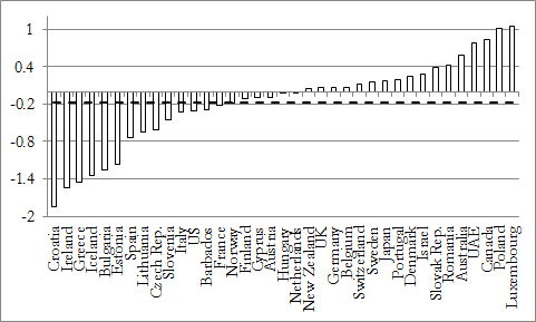
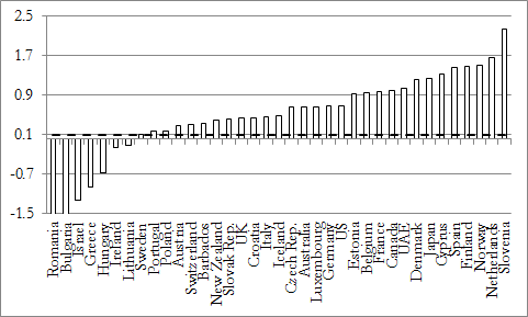 Figure 1: Government investment (left) and government consumption (right)
Source: Author’s calculations, using data from Gwartney et al. (2012) and World Bank’s World Develop-
ment Indicators. The dashed lines are the averages for all the countries.
Figure 1: Government investment (left) and government consumption (right)
Source: Author’s calculations, using data from Gwartney et al. (2012) and World Bank’s World Develop-
ment Indicators. The dashed lines are the averages for all the countries.